Constant rate birth (CRB) model • treepplr

library(treepplr)
library(ape)
library(ggplot2)
library(magrittr)

Data

We will use an example (random) tree that comes with the package.

tree <- ape::read.tree(system.file(
  "extdata/crb_tree_15_tips.tre", package = "treepplr"))
ape::plot.phylo(tree, cex = 0.5)
axisPhylo()

We need to convert the tree to a TreePPL readable format and read the CRB model.

data <- tp_phylo_to_tpjson(tree, age="tip-to-root")
model <- tp_model(system.file("extdata/crb.tppl", package = "treepplr"))

Run treeppl

Compile and run the TreePPL program with standard inference settings.

output_list <- tp_treeppl(model = model, data = data)

Plot posterior

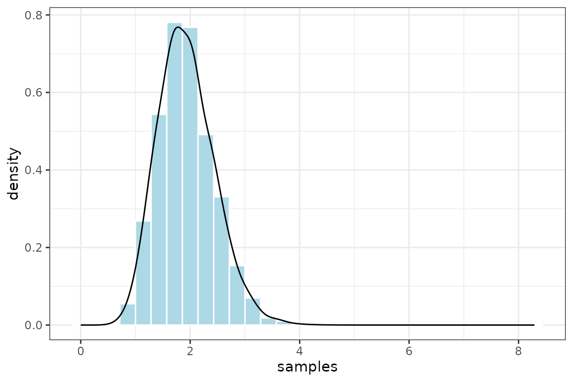
TreePPL outputs the log weight of each sample, so first we need to get the normalized weights and then we can plot the posterior distribution produced.

# turn list into a data frame where each row represents one sample 
# and calculate normalized weights from log weights and normalizing constants.
output <-  tp_parse(output_list) %>% 
  dplyr::mutate(total_lweight = log_weight + norm_const) %>% 
  dplyr::mutate(norm_weight = exp(total_lweight - max(.$total_lweight)))

ggplot2::ggplot(output, ggplot2::aes(samples, weight = norm_weight)) +
  ggplot2::geom_histogram(ggplot2::aes(y = ggplot2::after_stat(density)),
                 col = "white", fill = "lightblue", binwidth=0.04) +
  ggplot2::geom_density() +
  ggplot2::theme_bw()